
Notebook example
Galactic Velocity Curve Fit
Fit a sine curve to measured velocities and galactic longitudes.
Read the explanations, code, and available results below. Code does not run on this page.
The example uses sample measurements. Replace the CSV rows with your own observations to repeat the analysis.
Download sample data (CSV). Keep this file beside the notebook.
Run this notebook yourself
Use Python 3, Jupyter, NumPy, SciPy, and Matplotlib. Download the sample CSV alongside the notebook.
Download the notebook and open it in Jupyter. Review its code and data requirements before running the cells.
Sections in this example
Saved outputs are shown below.
Galactic Plane Sine Fit — Quadrants II & III
Companion analysis for the DSPIRA lesson Determining a Velocity Curve of the Milky Way Galaxy, Part 1: Galactic Quadrants II & III Observation.
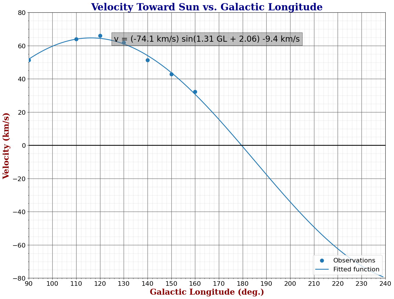
You have measured the Doppler velocity of the 21 cm hydrogen line at several galactic longitudes with the horn telescope. This notebook fits
$$v(\ell) = a \, \sin(b\,\ell + c) + v_\odot$$
to those measurements. A good fit is evidence that the Milky Way is rotating, and the sign of the fit tells you which way.
To use your own data: replace the numbers in quadrants_ii_iii_velocity_vs_longitude.csv
with your class's measurements, then re-run the notebook from the top.
import numpy as np
import matplotlib.pyplot as plt
from scipy.optimize import curve_fit
1. Load the observations
The data lives in a CSV next to this notebook so you can edit it without touching any code. Each row is one pointing: the galactic longitude you observed, and the velocity you derived from the Doppler shift of the HI peak.
DATA_FILE = "quadrants_ii_iii_velocity_vs_longitude.csv"

longitude_deg, velocity = np.loadtxt(DATA_FILE, delimiter=",", skiprows=1, unpack=True)
longitude_rad = np.radians(longitude_deg)

for l, v in zip(longitude_deg, velocity):
    print(f"  l = {l:5.1f} deg    v = {v:6.1f} km/s")
2. Fit a sine curve
V_SUN is the Sun's motion with respect to the Local Standard of Rest along this part of
the plane; the lesson treats it as a known offset rather than something we fit for. The
three free parameters are the amplitude a, the angular frequency b, and the phase c.
V_SUN = -9.4  # km/s, solar motion offset assumed by the lesson


def sine_model(longitude_rad, a, b, c):
    return a * np.sin(b * longitude_rad + c) + V_SUN


params, covariance = curve_fit(
    sine_model, longitude_rad, velocity, p0=[30, 2, 0]
)
a, b, c = params
errors = np.sqrt(np.diag(covariance))

print(f"amplitude a = {a:8.3f} +/- {errors[0]:.3f} km/s")
print(f"frequency b = {b:8.3f} +/- {errors[1]:.3f}")
print(f"phase     c = {c:8.3f} +/- {errors[2]:.3f} rad")
3. Plot the data and the fit
model_deg = np.arange(90, 240, 1.0)
model_velocity = sine_model(np.radians(model_deg), *params)

title_font = {"family": "serif", "color": "darkblue", "weight": "bold", "size": 24}
label_font = {"family": "serif", "color": "darkred", "weight": "bold", "size": 20}

fig, ax = plt.subplots(figsize=(16, 12))

ax.scatter(longitude_deg, velocity, s=80, zorder=3, label="Observations")
ax.plot(model_deg, model_velocity, lw=2, label="Fitted function")
ax.axhline(0, lw=2, color="black")

ax.set_title("Velocity Toward Sun vs. Galactic Longitude", fontdict=title_font)
ax.set_xlabel("Galactic Longitude (deg.)", fontdict=label_font)
ax.set_ylabel("Velocity (km/s)", fontdict=label_font)
ax.set_xlim(90, 240)
ax.set_ylim(-80, 80)

ax.xaxis.set_major_locator(plt.MultipleLocator(10))
ax.xaxis.set_minor_locator(plt.MultipleLocator(5))
ax.tick_params(labelsize=16)
ax.minorticks_on()
ax.grid(True, which="major", color="#666666", linestyle="-", linewidth=1)
ax.grid(True, which="minor", color="#999999", linestyle="-", alpha=0.2)

fit_info = f"v = ({a:.3g} km/s) sin({b:.3g} GL + {c:.3g}) {V_SUN:+.1f} km/s"
ax.text(
    0.5, 0.9, fit_info, transform=ax.transAxes, fontsize=20,
    ha="center", va="center",
    bbox=dict(boxstyle="square", facecolor="gray", alpha=0.5),
)
ax.legend(fontsize=16, loc="lower right")

fig.savefig("galactic_plane_sine_fit.png", dpi=150, bbox_inches="tight")
plt.show()
4. What does this tell us?
Questions for students:
- Every point in the sample data sits in quadrant II (galactic longitude 90-160 degrees) and every velocity is positive - hydrogen there is approaching us. What would you expect the sign to be in quadrant III, and why?
- The fitted curve crosses zero somewhere past 180 degrees, beyond where this data stops. What is physically happening at that longitude, and what observation would you need to make to check the prediction?
- How much does the fitted amplitude change if you drop your least confident data point? What does that say about how many pointings you need?