
Notebook example
Correlation and Interferometry
Explore convolution, autocorrelation, telescope beams, and interferometer fringes.
Read the explanations, code, and available results below. Code does not run on this page.
Pranav Sanghavi wrote the original material in 2018. The notebook was updated for Python 3 in 2026.
Run this notebook yourself
Use Python 3, Jupyter, NumPy, SciPy, and Matplotlib. No telescope or external data is needed.
Download the notebook and open it in Jupyter. Review its code and data requirements before running the cells.
Sections in this example
Saved outputs are shown below.
Correlation and the Two-Element Interferometer
Convolution, autocorrelation and cross-correlation, and what they have to do with putting two horn telescopes together.
Written by Pranav Sanghavi at the WVU Radio Astronomy Instrumentation Laboratory, 21 May 2018. Ported from Python 2 to Python 3 in 2026; the plots gained titles and axis labels, and the interactive widgets became ordinary figures so the notebook renders the same way everywhere.
Needs numpy, scipy and matplotlib and nothing else:
pip install numpy scipy matplotlib
jupyter notebook interferometry.ipynb
Every figure in this notebook is also generated by make_figures.py, which is
what the lesson page on the site uses.
On the u,v plane. The original notebook went on to aperture synthesis and u,v coverage, working through the excellent Fundamentals of Radio Interferometry course book from Rhodes University and NASSP. That part is not reproduced here — it is their material, under their licence, and their book explains it better than a copy of it would. Chapter 4, Visibility Space, is where to go next.
import numpy as np
import matplotlib.pyplot as plt
from scipy import signal

%matplotlib inline

# The notebook originally asked for the 'seaborn-poster' style. Matplotlib 3.6
# renamed every bundled seaborn style and 3.8 removed the old names, so asking
# for it by name now raises OSError.
for candidate in ("seaborn-v0_8-poster", "seaborn-poster"):
    try:
        plt.style.use(candidate)
        break
    except (OSError, ValueError):
        continue

plt.rcParams.update({
    "font.size": 13.0,
    "figure.dpi": 110,
    "axes.grid": True,
    "grid.alpha": 0.35,
    "axes.formatter.limits": (-7, 7),
    "axes.formatter.use_mathtext": True,
})
Convolution, Auto-correlation and Cross-correlation
Convolution
"In mathematics (and, in particular, functional analysis) convolution is a mathematical operation on two functions (f and g) to produce a third function, that is typically viewed as a modified version of one of the original functions, giving the integral of the pointwise multiplication of the two functions as a function of the amount that one of the original functions is translated" from wikipedia
$$ (f * g)(x) \,=\, \int_{-\infty}^{+\infty} f(x-t)\,g(t)\,dt $$
for multiple dimensions
$$ \begin{align} (f * g)(x_1,\ldots,x_n ) \,&=\, (f * g)({\bf x})\\ \,&=\, \int_{-\infty}^{+\infty} \ldots \int_{-\infty}^{+\infty} f(x_1-t_1, \ldots , x_n-t_n)\,g(t_1, \ldots, t_n) \,d^nt\\ \,&=\, \int_{-\infty}^{+\infty} f({\bf x}-{\bf t})\,g({\bf t}) \,d^nt\end{align} $$
Properties of convolution
$$ \begin{align} f * g \,&=\, g * f&\qquad (\text{commutativity})\\ (f * g)* h \,&=\, f * (g * h)&\qquad (\text{associativity})\\ f * (g + h) \,&=\, (f * g) + (f * h) &\qquad (\text{distributivity})\\ (a\, g) * h \,&=\, a \, (g * h)&\qquad (\text{associativity with scalar multiplication})\\ \end{align} $$
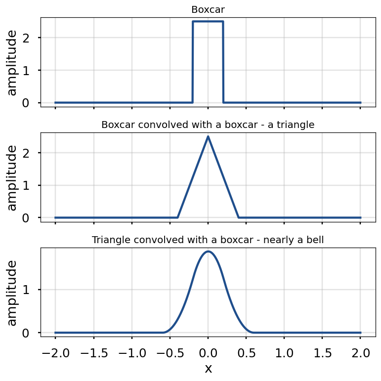
def boxcar(x, a, b, amp):
    """A rectangle of height `amp` between a and b."""
    return amp * np.logical_and(x >= a, x <= b)

a, b = -0.2, 0.2
xrange = [-2.0, 2.0]
xpoints = 1000
dx = (xrange[1] - xrange[0]) / float(xpoints)
x = np.linspace(xrange[0], xrange[1], xpoints)

# normalise to unit area so the three panels are comparable
y = boxcar(x, a, b, 1.0)
amp = float(xpoints) / ((xrange[1] - xrange[0]) * y.sum())
y = boxcar(x, a, b, amp)

once = dx * np.convolve(y, y, "same")
twice = dx * np.convolve(once, y, "same")

fig, axes = plt.subplots(3, 1, sharex=True, figsize=(7.2, 7.2))
for ax, data, title in zip(
        axes, (y, once, twice),
        ("Boxcar",
         "Boxcar convolved with a boxcar - a triangle",
         "Triangle convolved with a boxcar - nearly a bell")):
    ax.plot(x, data, "-", color="#1f4e8c")
    ax.set_title(title, fontsize=13)
    ax.set_ylabel("amplitude")
axes[-1].set_xlabel("x")
fig.tight_layout()
def gaussian(x, amp, mu, sigma):
    y = (x - mu) / sigma
    return amp * np.exp(-np.power(y, 2.0) / 2)

sigma = 0.1

def at(x0):
    """Index of position x0 in the x array."""
    return int((x0 - xrange[0]) / dx)

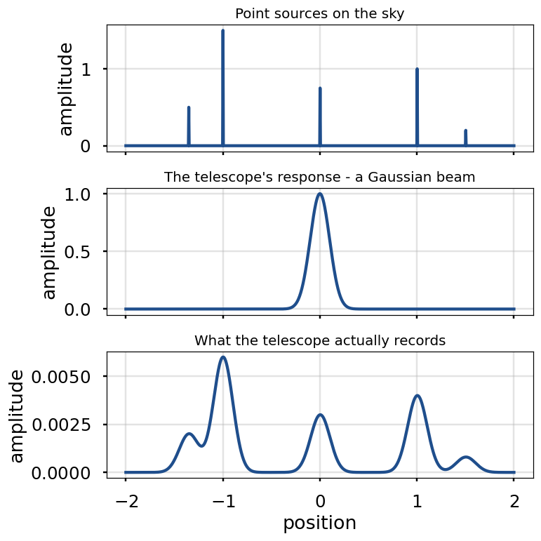
spikes = (signal.unit_impulse(xpoints, [at(-1.0), at(0.0), at(1.0)])
          + 0.20 * signal.unit_impulse(xpoints, at(1.50))
          - 0.25 * signal.unit_impulse(xpoints, "mid")
          + 0.50 * signal.unit_impulse(xpoints, at(-1.00))
          + 0.50 * signal.unit_impulse(xpoints, at(-1.35)))

kernel = gaussian(x, 1.0, 0.0, sigma)
smoothed = dx * np.convolve(spikes, kernel, "same")

fig, axes = plt.subplots(3, 1, sharex=True, figsize=(7.2, 7.2))
for ax, data, title in zip(
        axes, (spikes, kernel, smoothed),
        ("Point sources on the sky",
         "The telescope's response - a Gaussian beam",
         "What the telescope actually records")):
    ax.plot(x, data, "-", color="#1f4e8c")
    ax.set_title(title, fontsize=13)
    ax.set_ylabel("amplitude")
axes[-1].set_xlabel("position")
fig.tight_layout()
Cross-correlation
$$ \begin{split} (f\star g)(x) \,&=\, ({f_-}^*\circ g)(x)\\ &=\, \int_{-\infty}^{+\infty} f^*(t-x)\,g(t)\,dt\\ &\underset{t^\prime = t-x}{=}\, \int_{-\infty}^{+\infty} f^*(t^\prime)\,g(t^\prime+x)\,dt^\prime\\ \end{split}\qquad \text{,} $$
$$ \begin{align} (f\star g)(x_1,\ldots,x_n ) \,&=\, (f\star g)({\bf x})\\ &=\, ({f_-}^*\circ g)(x)\\ &=\, \int_{-\infty}^{+\infty} \ldots \int_{-\infty}^{+\infty} f^*(t_1-x_1, \ldots , t_n-x_n)\,g(t_1, \ldots, t_n) \,d^nt\\ \end{align} $$
Autocorrelation
$$ \begin{split} R\{f\}(x) \,&=\, (f\star f)(x)\\ &=\, (f_-^* * f)(x)\\ &=\, \int_{-\infty}^{+\infty} f^*(t-x)\,f(t)\,dt\\ &\underset{t^\prime = t-x}{=}\, \int_{-\infty}^{+\infty} f^*(t^\prime)\,f(t^\prime+x)\,dt^\prime\\ \end{split}\qquad \text{.} $$
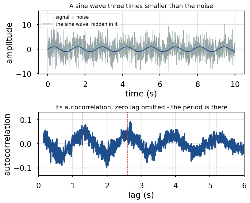
# Autocorrelation finds a periodicity you cannot see by eye.
rng = np.random.default_rng(20180521)
t = np.linspace(0, 10, 2000)
period = 1.3
clean = np.sin(2 * np.pi * t / period)
noisy = clean + rng.normal(0, 3.0, t.size)

ac = np.correlate(noisy, noisy, "full")[noisy.size - 1:]
ac = ac / ac[0]
lag = t - t[0]

fig, axes = plt.subplots(2, 1, figsize=(7.6, 6.2))
axes[0].plot(t, noisy, lw=0.7, color="#95a5a6", label="signal + noise")
axes[0].plot(t, clean, lw=1.6, color="#1f4e8c", label="the sine wave, hidden in it")
axes[0].set_xlabel("time (s)"); axes[0].set_ylabel("amplitude")
axes[0].set_title("A sine wave three times smaller than the noise", fontsize=13)
axes[0].legend(fontsize=10)

# Skip the zero-lag spike: it is 1.0 by construction and squashes everything
# that carries the information into the bottom of the panel.
keep = (lag >= 0.15) & (lag <= 6.0)
axes[1].plot(lag[keep], ac[keep], color="#1f4e8c")
for k in range(1, 5):
    axes[1].axvline(k * period, color="#c0392b", ls="--", lw=1)
span = np.abs(ac[keep]).max() * 1.35
axes[1].set_ylim(-span, span); axes[1].set_xlim(0, 6)
axes[1].set_xlabel("lag (s)"); axes[1].set_ylabel("autocorrelation")
axes[1].set_title("Its autocorrelation, zero lag omitted - the period is there",
                  fontsize=13)
fig.tight_layout()
Why Interferometry
HI_WAVELENGTH = 0.21   # m, the 21 cm line

def dish_diameter(angres_deg, wavelength=HI_WAVELENGTH):
    """Diameter needed for a given angular resolution, circular aperture."""
    return 1.22 * wavelength / np.radians(angres_deg)

for arcsec, what in [(3600.0, "1 degree"), (60.0, "1 arcmin"),
                     (1.0, "1 arcsec"), (0.015, "15 milliarcsec, the VLA")]:
    d = dish_diameter(arcsec / 3600.0)
    print("%-26s needs a dish %10.1f m across" % (what, d))

print("\nThe Earth is 12,742,000 m across.")
2 element interferometer
We can combine these signals:
- by addition to form a sum interferometer, or $\sum$-interferometer
- by multiplication to form a product interferometer, or $\prod$-interferometer.
The $\sum$-interferometer
$$P ={2 V_0^2(1+ \cos\Delta \Phi)} $$
The $\prod$-interferometer
$$R_c= \langle V_1 V_2 \rangle_t$$ $$R_c =\frac{V_0^2}{2}\cos{\omega \tau}=\frac{V_0^2}{2}\cos \Delta \Phi$$ where $\tau$ is the time delay in the signal path
This is a cosine correlator, one can consider a sine correlator by introducing an artificial phase delay of $\frac{\pi}{2}$ in one of the two signal paths:
$$V_1=V_{01} \cos (\omega (t + \tau)) \quad V_2 = V_{02} \cos (\omega t + \frac{\pi}{2} )$$
\begin{eqnarray} R&=&\langle V_{01} V_{02} \cos{(\omega t + \frac{\pi}{2})} \cos{[\omega (t + \tau) ]} \rangle_t\\ R&=& V_0^2 \frac{\langle \cos(2 \omega t + \tau + \frac{\pi}{2})+\cos (\omega \tau - \frac{\pi}{2})\rangle_t}{2} \end{eqnarray} $$R_s =\frac{V_0^2}{2}\sin{\omega \tau}$$
we can combine the two operations to obtain a complex correlator
$$R = \int_{\Omega} I_\nu(\mathbf{s}) e^{-\imath 2\pi \frac{\mathbf{b}\cdot\mathbf{s}}{\lambda}} d\Omega = V$$
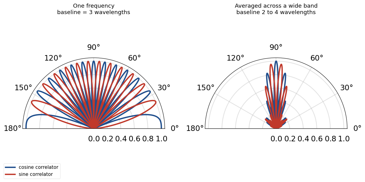
theta = np.linspace(0.0, 180.0, 1000)

# a single frequency, baseline three wavelengths long
single = np.exp(-1j * 2 * np.pi * 3.0 * np.cos(np.radians(theta)))

# the same baseline seen across a wide band, 2 to 4 wavelengths
blambda = np.linspace(2.0, 4.0, 100)
wide = np.zeros_like(theta, dtype=complex)
for bl in blambda:
    wide += np.exp(-1j * 2 * np.pi * bl * np.cos(np.radians(theta)))

single = single / np.abs(single).max()
wide = wide / np.abs(wide).max()

fig, axes = plt.subplots(1, 2, figsize=(11.0, 5.4),
                         subplot_kw={"projection": "polar"})
for ax, data, title in zip(
        axes, (single, wide),
        ("One frequency\nbaseline = 3 wavelengths",
         "Averaged across a wide band\nbaseline 2 to 4 wavelengths")):
    ax.plot(np.radians(theta), np.abs(np.real(data)),
            color="#1f4e8c", label="cosine correlator")
    ax.plot(np.radians(theta), np.abs(np.imag(data)),
            color="#c0392b", label="sine correlator")
    ax.set_title(title, fontsize=12, pad=18)
    ax.set_thetamin(0); ax.set_thetamax(180)
axes[0].legend(loc="lower left", bbox_to_anchor=(-0.15, -0.12), fontsize=10)
fig.tight_layout()
Effect of Bandwidth
Credits and reuse
The text and code above are Pranav Sanghavi's, written for the WVU Radio Astronomy Instrumentation Laboratory in 2018, and are published here under the same MIT licence as the rest of this repository. The autocorrelation figure was added in 2026; everything else is his.
The Wikipedia definition of convolution quoted at the top is used under CC BY-SA 4.0.
For aperture synthesis, u,v coverage and everything that follows from two elements to an array, go to Fundamentals of Radio Interferometry (Rhodes University / NASSP, GPL v2) — chapter 4 in particular. It is free to read online and is the standard text for this material.