Notebook example
Green Bank Telescope Drift Scan
Read the 2017 observation and its ten preserved plots.
Read the explanations, code, and available results below. Code does not run on this page.
The ten plots shown here come from the original 2017 run. They have not been recomputed.
The original HDF5 dataset is missing, so this notebook cannot currently be rerun as supplied.
Frequency conversion, clock correction, and integration ranges are specific to the GBT observation. Adapt them before analyzing another dataset.
Run this notebook yourself
Use Python 3, Jupyter, NumPy, Matplotlib, and h5py. The original HDF5 dataset is unavailable.
Download the notebook and open it in Jupyter. Review its code and data requirements before running the cells.
Sections in this example
Saved outputs are shown below.
GNU Radio and GBT
The RET-DSPiRA cohort of 2017 had the unique opportunity of using their own DSP spectrometer program they designed in GNU Radio to process signal from the Green Bank Telescope. We tapped into the Green Bank Telescope IF signal to the Airspy sdr dongle and recorded a drift scan with the GBT in the L-band. The VEGAS spectrometer back end usually fully connected from the IF rack had one of the polarizations sent to the tapped port. VEGAS also simultaniousy took the data. This notebook reduces the data taken. Feel free to download it and play around with it if you like.
Before pointing this at your own data: three things here are specific to this one 2017 GBT observation. The frequency axis is rebuilt as
1670.4e6 - (...)— that undoes the GBT's intermediate-frequency downconversion, and a horn telescope's file needs the plainnp.arange(flength)*fstep + fstartinstead. The timestamps get+ 43200— a half-day correction for a clock that was set wrong that day; your data does not want it. And several cells slice fixed integration ranges (spec[300:400],spec[7500:9700]) that only exist in this 19,280-integration file. Read it as a worked example of the method — the calibration against the noise diode is the part that transfers.
%matplotlib inline
!ls -ltrh ## the folder where the data is
############## Import Packages
import h5py
import matplotlib.pylab as plt
import numpy as np
from datetime import datetime

############# Random stuff to prettify the plots :3
plt.rcParams['figure.figsize'] = [8.4, 6.8]
plt.rcParams['font.family'] = ['serif']
plt.rcParams['xtick.major.size'] =  6
plt.rcParams['ytick.major.size'] =  6
plt.rcParams['xtick.minor.size'] =  3
plt.rcParams['ytick.minor.size'] =  3
plt.rcParams['lines.linewidth'] = 1
plt.rcParams['mathtext.fontset'] = 'cm'
plt.rcParams['xtick.direction'] = 'out'
plt.rcParams['ytick.direction'] = 'out'
plt.rcParams['xtick.top'] = False
plt.rcParams['ytick.right'] = True
###################################################################################################################
########                        import the hdf5 file of the data in question                                #######
###################################################################################################################
f = h5py.File('/home/dspradio/grc_data/2017-08-01_09.25.56_GBTdrift.h5','r')
###################################################################################################################
########                                  List all the data metadata                                        #######
###################################################################################################################
list(f.attrs.items())
###################################################################################################################
########                                 List the data Heirarchies                                          #######
###################################################################################################################
list(f.items())
###################################################################################################################
########                 extract the spectroeter data and timestamps                                        #######
###################################################################################################################
spec = f['spectrum'][:,:]
tunix = f['timestamp'][:] + 43200 #  my system time was 12 hrs behind so added 12 hours to time!)
###################################################################################################################
########                        convert the unix timestamp to human date                                    #######
###################################################################################################################
print("Observation Started on " + datetime.fromtimestamp(f.attrs['start_time']).strftime('Date: ''%Y-%m-%d' ' Time: ' '%H:%M:%S') )
print("Observation Ended on " + datetime.fromtimestamp(tunix[-1]).strftime('Date: ''%Y-%m-%d' ' Time: ' '%H:%M:%S') )

t = []  # make a list of human readable time of integration point

### List of human readable integration timestamps
for i in tunix: t.append(datetime.fromtimestamp(int(i)).strftime('%Y-%m-%d %H:%M:%S'))

### Hours Observed
hobs = (tunix[-1]-tunix[0])/3600
s = 'Hours Observed = ' + repr(hobs[0])
print(s)
###################################################################################################################
########                                                                                                    #######
###################################################################################################################
fstart = f.attrs['freq_start']       # get the start frequency
fstep = f.attrs['freq_step']         # get the stop frequency
flength = 4096                       # the number of points on the frequency axis, vector length
freq = 1670.4e6 - (np.arange(flength)*fstep + fstart)         # make an array of x-axis indices value
freqghz = freq/10e8 # scaled to mark axis
The Data
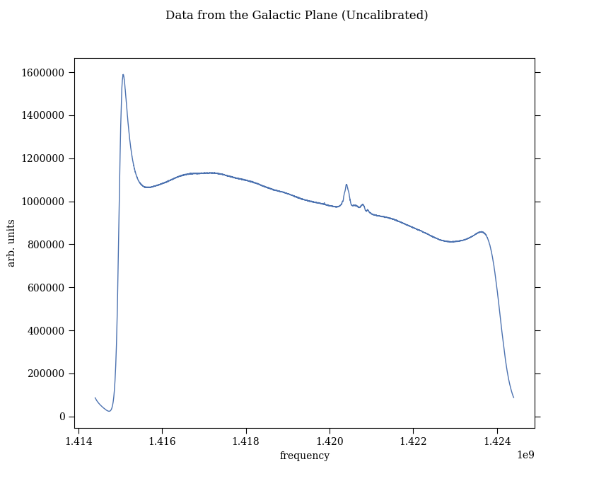
plt.figure()
plt.suptitle("Data from the Galactic Plane (Uncalibrated)")
plt.ylabel("arb. units")
plt.xlabel("frequency")
plt.plot(freq,np.mean(spec[8000:8250],axis=0))
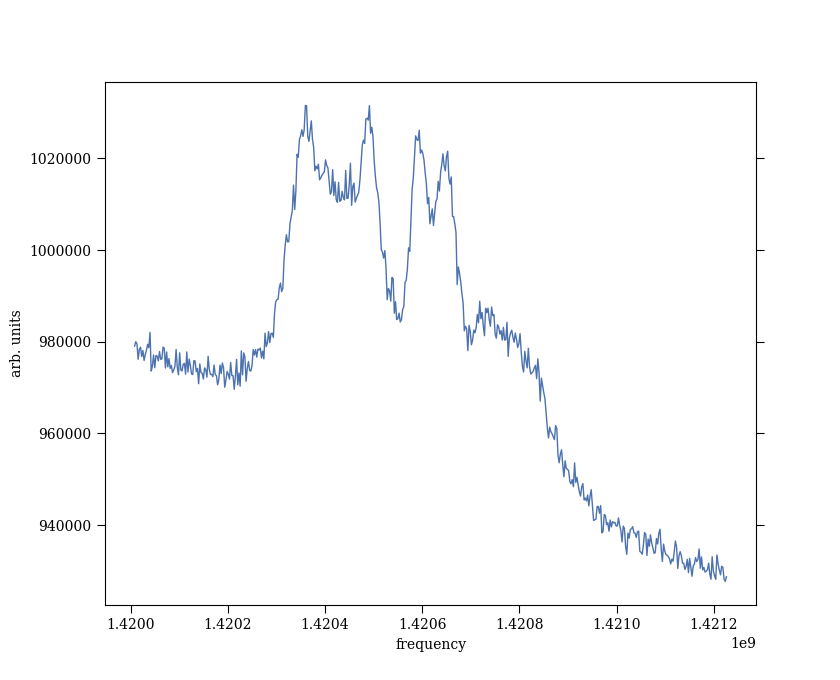
plt.figure()
plt.ylabel("arb. units")
plt.xlabel("frequency")
plt.plot(freq[1300:1800],np.mean(spec[9150:9200,1300:1800],axis=0))
Calibration
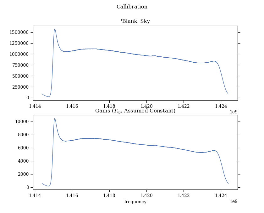
To have our data make physical sense need to calibrate the data. In practice the GBT has a noise diode injecting a known noise to the signal switching on and off continuously through time. But we did not have that for our setup. We will make some assumptions.
$$ power = g(T_{sky}+T_{sys}) \\ T_{sys} = assume( 143 K) $$
From GBT systems, usually around 20K but maintenance stuff added extra temp. this night
$$ T_{sky} = assume( 7 K)\\ gains = \frac{power}{T_{sky}+T_{sys}} \\ T_{sky} = \frac{p}{gains} - T_{sys} $$
###################################################################################################################
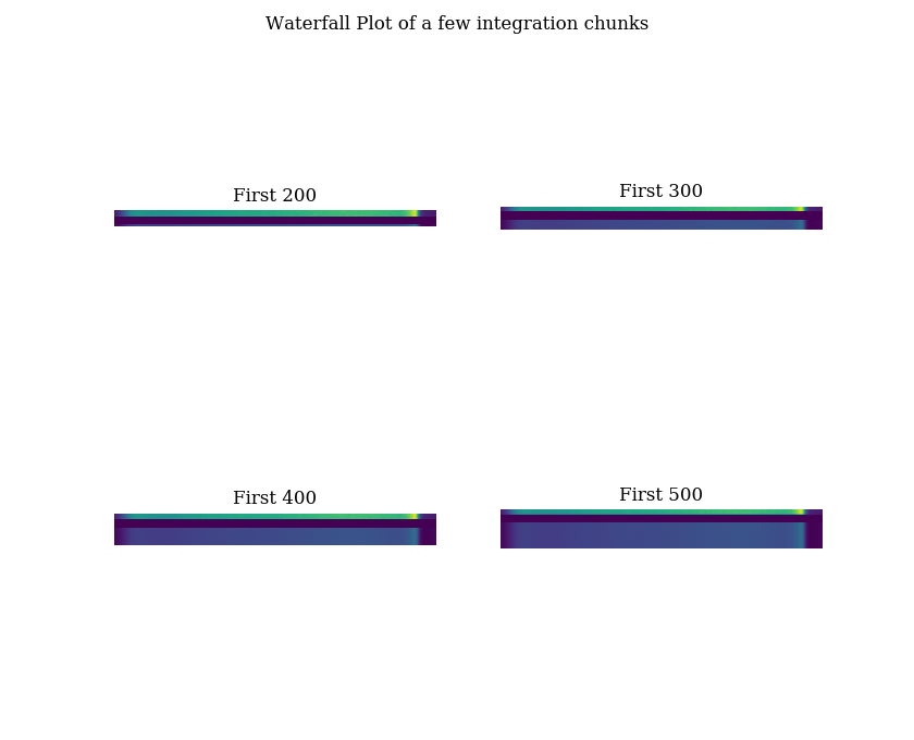
###############             Check waterfall to look for the empty sky spectrum                   ##################
###############        the first 200 or so integrations there were probelms in the gbt backend   ##################
###################################################################################################################
s200 = spec[0:200]
s300 = spec[0:300]
s400 = spec[0:400]
s500 = spec[0:500]
plt.figure()
plt.suptitle("Waterfall Plot of a few integration chunks")
plt.subplot(221)
plt.title("First 200")
plt.axis('off')
plt.imshow(s200)
plt.subplot(222)
plt.title("First 300")
plt.axis('off')
plt.imshow(s300)
plt.subplot(223)
plt.title("First 400")
plt.axis('off')
plt.imshow(s400)
plt.subplot(224)
plt.title("First 500")
plt.axis('off')

plt.imshow(s500)
#########################################################################################################
############                  Caliberate!                                         #######################
#########################################################################################################

plt.figure()

plt.suptitle("Callibration")
plt.subplot(211)
plt.title("'Blank' Sky")
plt.plot(freq,np.mean(spec[300:400],axis = 0))

tsys = 143.5
tsky = 7

T = tsys+tsky

psky = np.mean(spec[300:400],axis = 0)
g = psky/T

plt.subplot(212)
plt.title("Gains ($T_{sys}$ Assumed Constant)")
plt.xlabel("frequency")
plt.plot(freq,g)

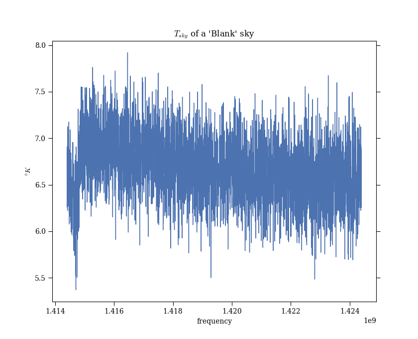
plt.figure()
plt.title("$T_{sky}$ of a 'Blank' sky ")
spectrum = (spec[400:500]/g) - tsys
plt.ylabel("$ \degree K $")
plt.xlabel("frequency")
plt.plot(freq,np.mean(spectrum,axis=0))

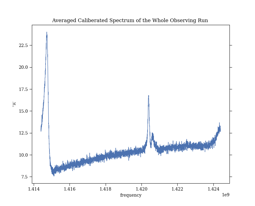
spectrumcal = (spec/g) - tsys
plt.figure()
plt.title("Averaged Caliberated Spectrum of the Whole Observing Run ")
plt.ylabel("$ \degree K $")
plt.xlabel("frequency")
plt.plot(freq,np.mean(spectrumcal,axis=0))
plt.figure()
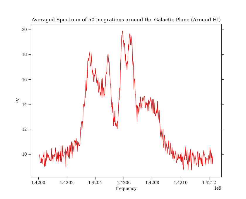
plt.ylabel("$ \degree K $")
plt.xlabel("frequency")
plt.title("Averaged Spectrum of 50 inegrations around the Galactic Plane (Around HI)")
plt.plot(freq[1300:1800],np.mean(spectrumcal[9150:9200,1300:1800],axis=0), 'r')

plt.figure()

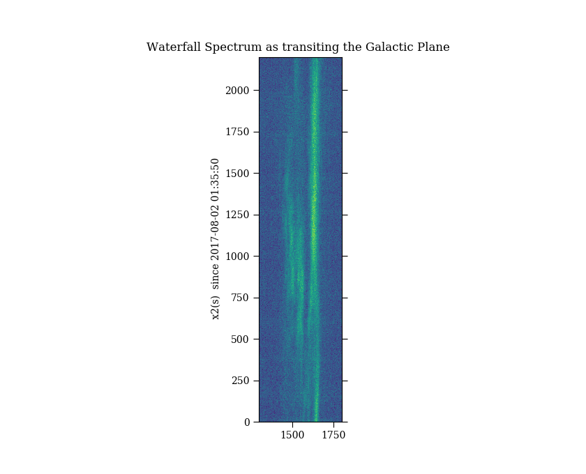
plt.title("Waterfall Spectrum as transiting the Galactic Plane ")
plt.ylabel(" x2(s)  since " + str(t[7500]))
plt.imshow(spectrumcal[7500:9700, 1300:1800], extent=[1300,1800,7500-7500,9700-7500])
plt.figure()
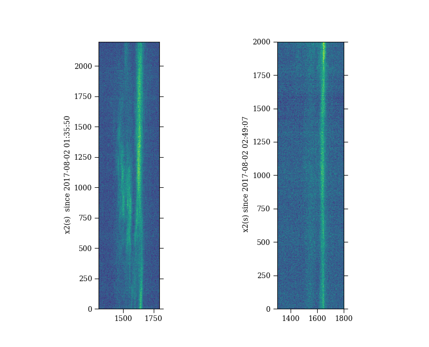
plt.subplot(1,2,1)
plt.imshow(spectrumcal[7500:9700, 1300:1800], extent=[1300,1800,(7500-7500),(9700-7500)])
plt.ylabel(" x2(s)  since " + str(t[7500]))
plt.subplot(1,2,2)
plt.ylabel(" x2(s) since " + str(t[9700]))
plt.imshow(spectrumcal[9700:11700, 1300:1800], extent=[1300,1800,(9700-9700),(11700-9700)])
plt.figure()
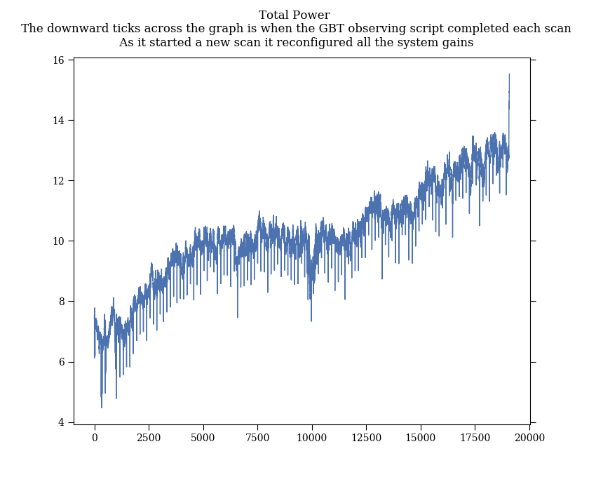
plt.suptitle("Total Power\n The downward ticks across the graph is when the GBT observing script completed each scan\n As it started a new scan it reconfigured all the system gains")
plt.plot(np.mean(spectrumcal[200:],axis=1))