I/Q Quadrature Sampling

%matplotlib inline
import numpy as np
from matplotlib.pyplot import *

# Setup constants
Nx = 65536  #Large number of samples
Fs = 200e6  #Sampling frequency
Flo = 1.4e9 #Frequency 'tuned' to.
F1 = 1.42e9 # Input tone we're trying to listen to
F2 = 1.38e9 # other tone we're trying to listen to
fs_rf = 12e9 # Frequency running simulation at.
freq = np.fft.fftfreq(Nx,1.0/(fs_rf/1e6))
signal1 = np.cos(2.0*np.pi * F1/fs_rf * np.arange(Nx))# + 0.03)  # make the 1.42MHz tone
signal2 = np.cos(2.0*np.pi * F2/fs_rf * np.arange(Nx))# + 0.05 ) # make the 1.38MHz tone
signal_loI = np.cos(2.0*np.pi * Flo/fs_rf * np.arange(Nx) ) #make the signal from the receiver to 'tune'
signal_loQ = np.sin(2.0*np.pi * Flo/fs_rf * np.arange(Nx) ) #make the signal from the receiver to 'tune'

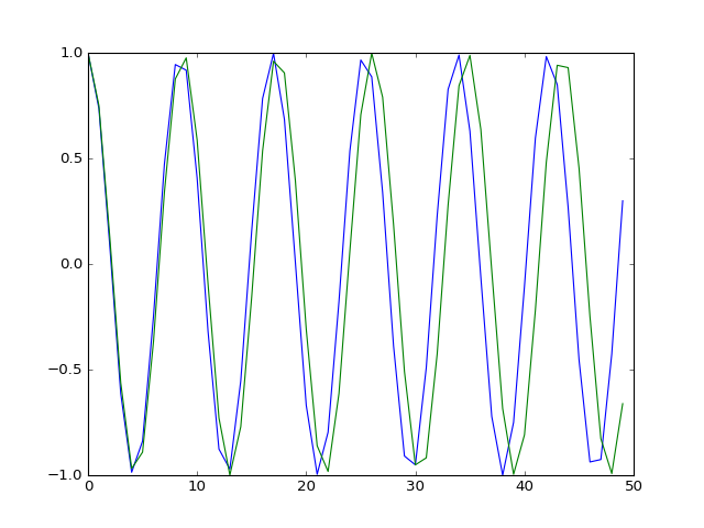
#Plot the 2 incoming tones.
figure()
plot(signal1[:50])
plot(signal2[:50])

# Put the input signals into the Receiver for Mixing, where multiply by a cosine and a sine
mixed1I = signal1 * signal_loI
mixed1Q = signal1 * signal_loQ
mixed2I = signal2 * signal_loI
mixed2Q = signal2 * signal_loQ

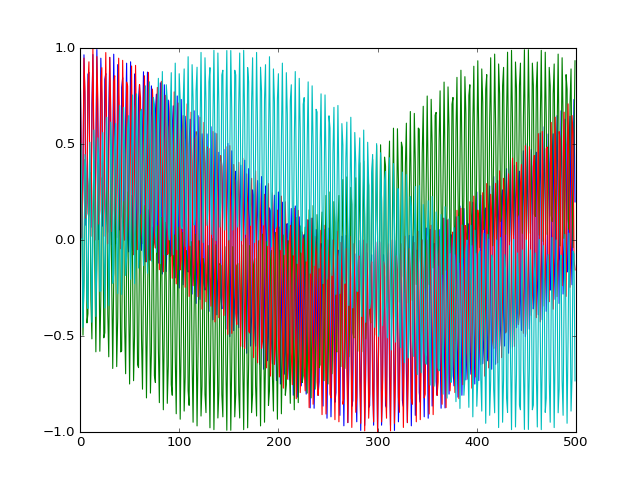
# Observer that we now have both the 'slow' 20 MHz (difference) and fast ~2.8GHz signals
figure()
plot(mixed1I[:500])
plot(mixed1Q[:500])
plot(mixed2I[:500])
plot(mixed2Q[:500])

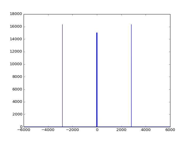
#Observe just the "I" output has 2 positive and 2 negative tones visible(low freq hard to see there are 2)
#after mixing the 'zero' is relative to the "LO" or receiver tuned frequency.
figure()
plot(freq, np.abs(np.fft.fft(mixed1I)))

# Hard fourier cutoff lowpass filter.  This is the same as a 'rectangular' window in fourier space.
# This would usually be an analog filter of some kind in the receiver.
figure()
N_cutoff = int(Fs/fs_rf*Nx)
signals = [mixed1I, mixed1Q, mixed2I, mixed2Q]
filtered_signals = []

#Now can observe there are only the 'low frequency' positive and negative 20MHz tones

for signal in signals:
    fsignal = np.fft.fft(signal)
    fsignal[N_cutoff:-N_cutoff] = 0.0
    plot(freq, abs(fsignal))
    filtered_signals.append(np.fft.ifft(fsignal))
    
xlim(-200,200)

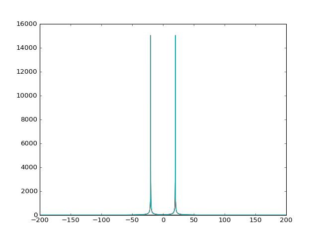
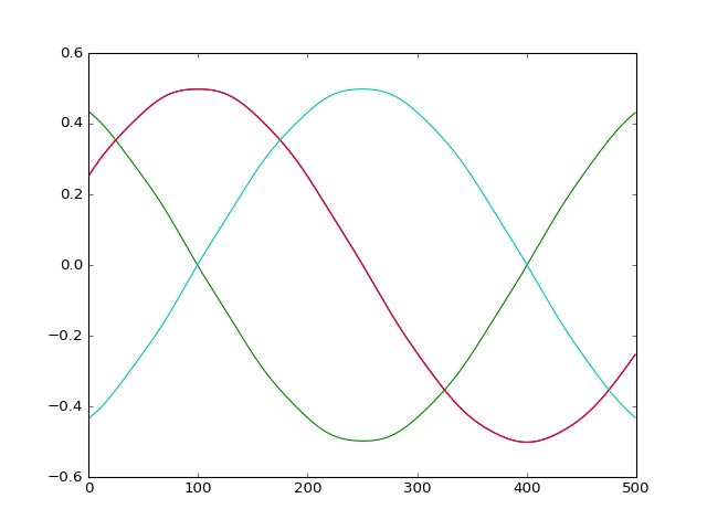
# Observer the timeseries again.  Now only have the 'slow' frequencies
# Notice however there are now 2 totally in phase, and 2 180 out of phase.  
figure()
for signal in filtered_signals:
    plot(signal[500:1000])

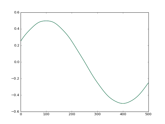
# "I" part is exactly the same for both the 1.38 and 1.42GHz signals
figure()
plot(filtered_signals[0][500:1000])
plot(filtered_signals[2][500:1000])

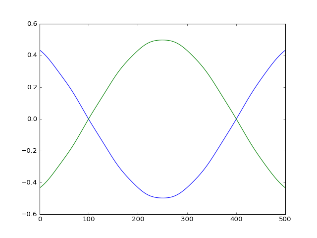
# "Q" part is exactly 180 out of phase for the 1.38 and 1.42GHz signals
figure()
plot(filtered_signals[1][500:1000])
plot(filtered_signals[3][500:1000])

# Make the 'complex' signal I - j*Q.  
#
s1 = filtered_signals[0] - 1.0j*filtered_signals[1]
s2 = filtered_signals[2] - 1.0j*filtered_signals[3]

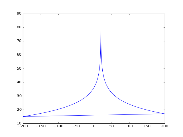
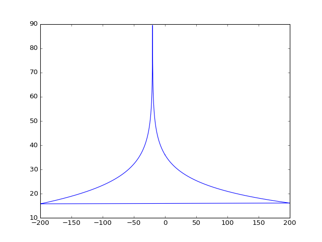
# Now can just take the fourier transform of the IQ quadrature signal we've just created and recover the 'original' 
# spectrum shifted down by 1.4GHz.
# 0 Frequency corresponds to 1.4GHz.  -20MHz is 1.38GHz, 20MHz is 1.42GHz.
figure()
freq = np.fft.fftfreq(Nx,1.0/(fs_rf/1e6))
slices = np.concatenate((np.arange(1092), np.arange(Nx-1092,Nx,1)))
print(slices)
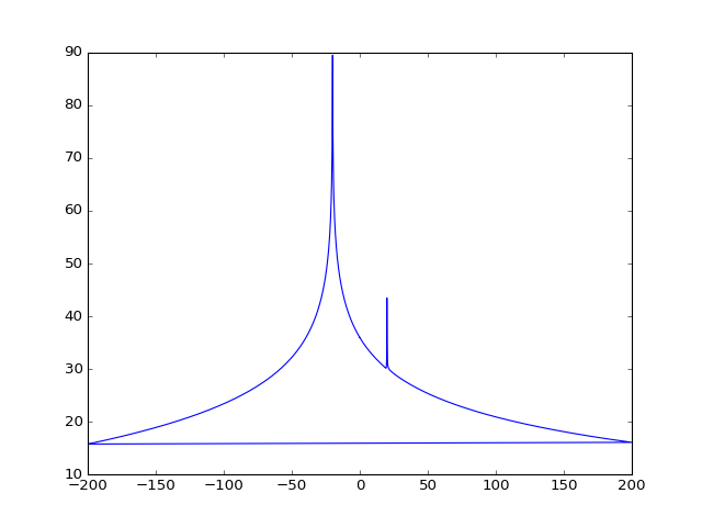
plot(freq[slices],20*np.log10(abs(np.fft.fft(s1))[slices]))
#Can recover just the +20MHz signal

#Can recover just the -20MHz signal.
figure()
plot(freq[slices],20*np.log10(abs(np.fft.fft(s2))[slices]))

#Of course the I and Q pass through different analog filters/amplifiers/mixers and ADC
# The I and Q signal will be off by a bit.  

#Let's simulate that.
imbalanced = [0.99*signal1 * signal_loI, signal1 * signal_loQ, 0.99*signal2 * signal_loI, signal2 * signal_loQ]

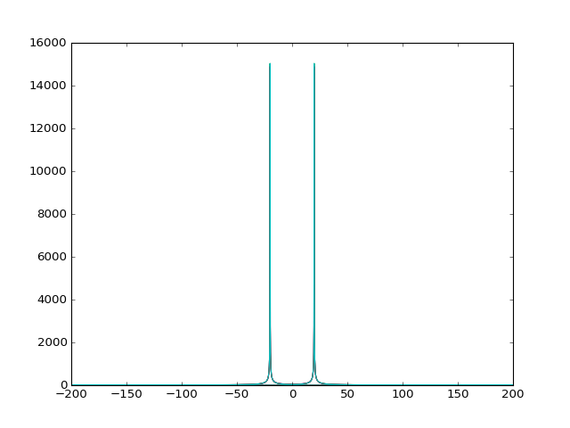
#Filter and plot the unbalanced signals.  Not obviously different...
figure()
filtered_signals_imbalanced = []
for signal in imbalanced:
    fsignal = np.fft.fft(signal)
    fsignal[N_cutoff:-N_cutoff] = 0.0
    plot(freq, abs(fsignal))
    filtered_signals_imbalanced.append(np.fft.ifft(fsignal))
xlim(-200,200)

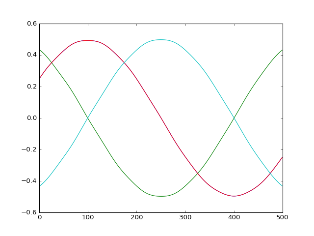
# Also un-noticeable in the time domain.
figure()
for signal in filtered_signals_imbalanced:
    plot(signal[500:1000])

# Create 'complex' IQ sampling output again.  Rember this is what an SDR dongle
#gives as an output for processing by GNU Radio.
s1im = filtered_signals_imbalanced[0] - 1.0j*filtered_signals_imbalanced[1]
s2im = filtered_signals_imbalanced[2] - 1.0j*filtered_signals_imbalanced[3]

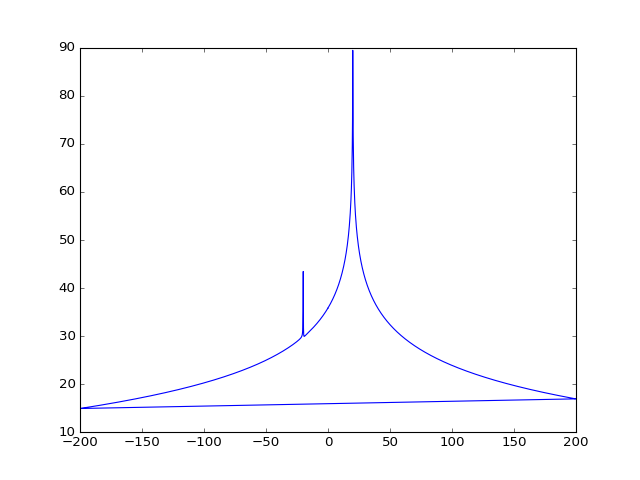
# Now what should be a pure tone at 20MHz also has a small one at -20MHz.  This is non-ideal when trying to measure a pure signal.  
figure()
plot(freq[slices],20*np.log10(abs(np.fft.fft(s1im))[slices]))

#Same for the -20MHz.  
figure()
plot(freq[slices],20*np.log10(abs(np.fft.fft(s2im))[slices]))