Running the Calibrated Spectrometer

Current software uses applications/spectrometry/calibrated-spectrometer.grc. Older videos and bootable images call it spectrometer_w_cal.grc.

The video shown here explains the features in this program.

Before Starting The Program

The video here explains how set up the horn and make adjustments to the user-defined settings referred to below.

• Check the user-defined settings illustrated below. These are the Variable blocks in the upper right corner of the GNU Radio canvas.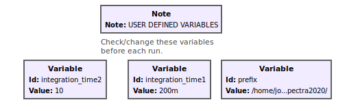

  

  • Double-click the box, enter a new value in the Value box, and click OK.

  • integration_time1 is the short integration time, and integration_time2 is the long integration time. These can be changed to any value at 0.4 s or above.

  • Check the prefix variable before recording. It combines the output folder with an optional filename prefix.

    Current application downloads use your home folder and begin filenames with spectrum_. Follow the software guide to choose a folder with DSPIRA_OUTPUT_DIR. Create that folder before launching GNU Radio Companion.

    You can also edit prefix directly. Enter an absolute path inside quotes, such as "/home/jansky/horn_data/spectrum_". Replace the example with your own existing, writable folder. Use a trailing slash instead of spectrum_ if you want filenames to begin with the timestamp.

    Older images and videos may show a different default path. Check your installed flowgraph before collecting data.

• CAUTION: Plug your laptop into power. Otherwise, it may enter sleep mode and stop the program during a long run. Change the power settings on your computer so that it never suspends or goes to sleep.

After Starting The Program

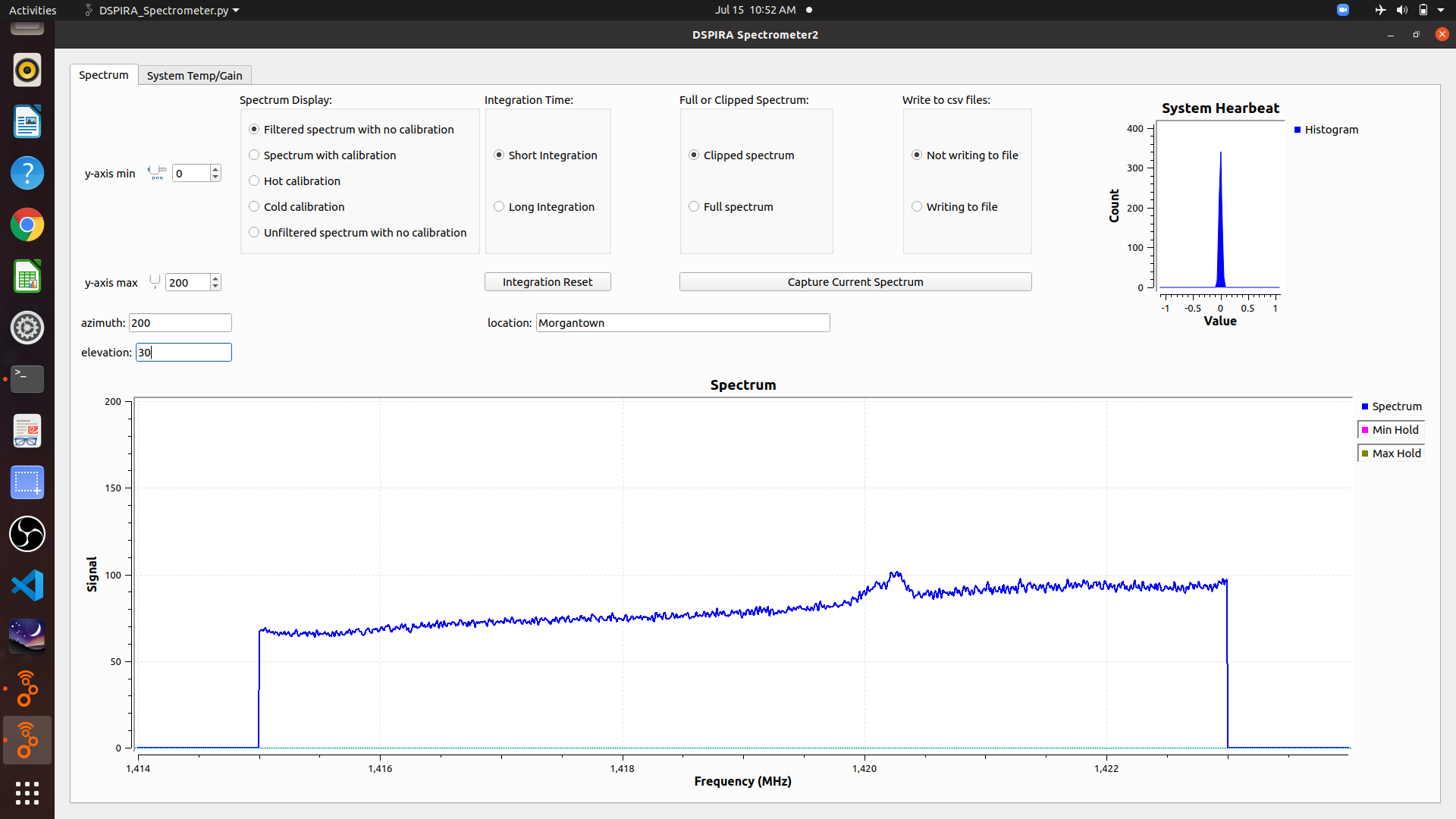
• The first screen that appears looks like the following:

• This display is used for most observations that are uncalibrated.

• Adjust the ymin and ymax values to scale the graph as desired.

• Fill in the azimuth, elevation, and location, if desired.

  • NOTE: Press ENTER after each value so the program records it.

  • These parameters are included in the title, as described in the Saving a Spectrum to a Data File section below. This is also demonstrated in this video..

• The Short Integration option is good for quick observations and demonstrations. Once the pointing is settled, switch to Long Integration for a longer run with smoother data.

• The Clipped Spectrum is the better selection for most viewings. The Full Spectrum is good for demonstrating how the signal processing affects the spectrum. It also might be useful for the expert user who wants the full spectrum for some reason.

Saving a Spectrum to a Data File

• Video - describes how to save data

• Click Capture Current Spectrum to save the displayed spectrum as a .csv data file. The data file is written to the folder under the path in the prefix Variable box.

• Select Writing to file under Write to csv File. The program then creates a new file in the data folder after each integration period. For instance, if Long Integration is selected and is 10 s, then every 10 s a new file is written. So for a 20 minute run, a total of 120 files will be written to the data folder.

Use this option for drift scans or unattended observations scheduled for later.

• Data File Format:

  • The .csv format is a .txt data file that can be opened in any spreadsheet.

  • When opened in a spreadsheet, the data will appear in 2 columns. The first column contains frequency in MHz. The recorded band depends on your receiver settings. The second column is the signal.

  • A graph of Signal vs. Frequency can easily be created after opening a file in a spreadsheet.

  • The file name has a format that contains the date, time, location, azimuth, and elevation, with “_spectrum” at the end. The location, azimuth, and elevation are recorded with the values in the corresponding fields on the spectrometer interface screen.

  • For example, 2020-07-15_12.30.00.000001_Morgantown_200_30_spectrum.csv identifies data collected in Morgantown on July 15, 2020. The telescope pointed at azimuth 200 degrees and elevation 30 degrees.